Tests using Biexponential model

The biexponential model outputs a sum of exponentials:

\[M(t) = A_1 \exp{(-R_1 t)} + A_2 \exp{(-R_2 t)}\]

The model parameters are the amplitudes \(A_1\), \(A_2\) and the decay rates \(R_1\) and \(R_2\).

Although the model is straightforward it can be challenging as an inference problem as the effect of the two decay rates on the output is nonlinear and can be difficult to distinguish in the presence of noise.

Test data

For testing purposes we define the ground truth parameters as:

• \(A_1=10\)
• \(A_2=10\)
• \(R_1=1\)
• \(R_2=10\)

The variables within the test data are:

• The level of noise present. For this test data we use Gaussian noise with a standard deviation of 1.0.
• The number of time points generated. We generate data sets with 10, 20, 50 and 100 time points (in each case the value of \(t\) ranges from 0 to 5 so only the data resolution changes in each case)

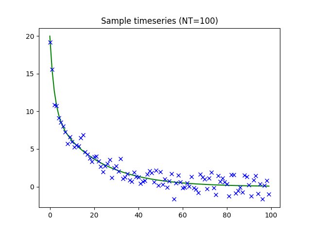
An example timeseries with these parameters is show below (100 time points, ground truth overlaid on noisy data):

1000 timeseries instances were generated and used for each test.

One issue with the biexponential model is that there are always two equivalent solutions obtained by exchanging \(A_1, R_1\) with \(A_2, R_2\). To prevent this from confusing reports of mean parameter values, we normalize the results of each run such that in each voxel \(A_1, R_1\) is the exponential with the lower rate.

Test variables

The following variables were investigated

• The learning rate
• The size of the sample taken from the posterior when set independently of the batch size
• The batch size when using mini-batch processing (NB this cannot exceed the number of time points)
• The prior distribution of the parameter
• The initial posterior distribution of the parameters
• The use of the numerical (sample-based) calculation of the KL divergence on the posterior vs the analytic solution (possible in this case only because both prior and posterior are represented by a multivariate normal distribution).
• Whether covariance between parameters is modelled. The output posterior distribution can either be modelled as a full multivariate Gaussian with covariance matrix, or we can constrain the covariance matrix to be diagonal so there is no correlation between parameter values.

We investigate convergence by calculating the mean of the cost function across all test instances by epoch. Note that this measure is not directly comparable when different priors are used as the closeness of the posterior to the prior is part of the cost calculation. Convergence is plotted by runtime, rather than number of epochs for two reasons: Firstly since this is the measure of most interest to the end user, and also because in the case of mini-batch processing one epoch may represent multiple iterations of the optimization loop.

We also consider per-voxel speed of convergence, defined for each voxel as the epoch at which it first came within 5% of its best cost. This definition is only useful when convergence was eventually achieved.

Effect of learning rate

The learning rate determines the size of optimization steps made by the gradient optimizer and can be a difficult variable to select. Too high and the optimizer may repeatedly overshoot the minima and never actually converge, too low and convergence may simply be too slow. In many machine learning problems the learning rate is determined by trial and error however in our case we do not have this luxury as we need to be able to converge the model fitting on any unseen data without user intervention.

The convergence of the mean cost is shown below by learning rate and number of time points. In these tests mini-batch processing was not used, the analytic calculation of the KL divergence was used and the posterior sample size was 200.

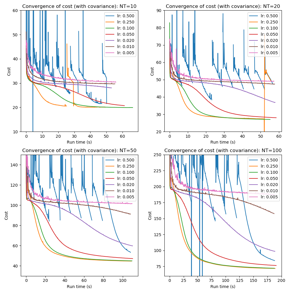
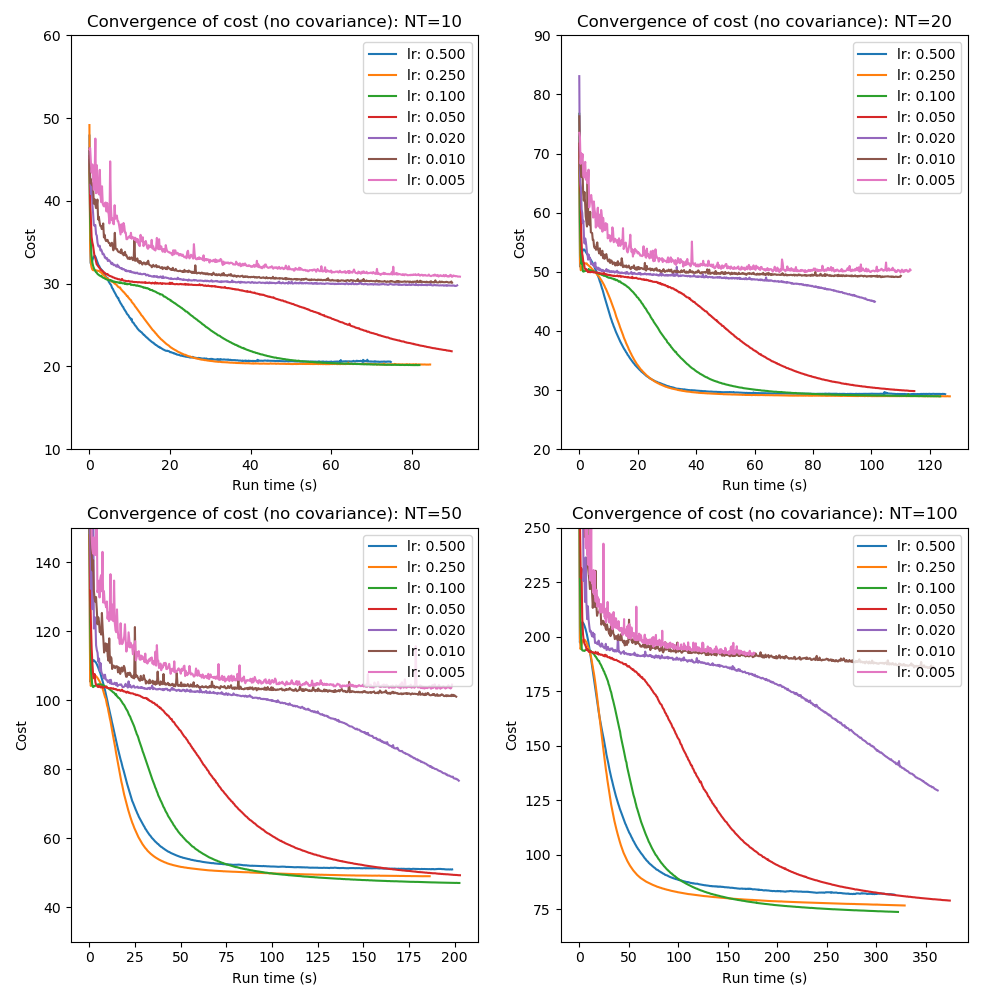
Although the picture is rather messy some observations can be made:

• Excessively high learning rates are unstable and do not achieve the best cost across the data sets (a learning rate of 1.0 was also tested but not plotted as the instability made the plots difficult to read).
• Very low learning rates (0.02 or lower) converge too slowly to be useful
• Even some learning rates which appear to show good smooth convergence do not achieve the minimum cost (e.g. LR=0.25, the amber line on some plots)
• Convergence with covariance is much more challenging as would be expected since the total number of fitted parameters rises from 10 to 20 per instance. In this high-dimensional space finding the overall cost minimum is likely to be more difficult.
• A learning rate of 0.1 gives the fastest reliable convergence. We will use this learning rate in subsequent tests where a single learning rate is required.
• Nevertheless initial convergnce can be faster at a higher learning rate (0.25 or 0.5) suggesting use of ‘quenching’ where the learning rate is decreased during the optimization.

We can also examine the best cost achieved at various learning rates including variation in the posterior sample size:

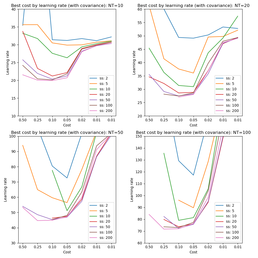
These plots reinforce that a learning rate of 0.1 seems optimal for attaining best cost across a range of tests although there may be slight benefit to a higher rate when including covariance.

Increasing the posterior sample size leads to a gradual lowering of the best cost with little improvement beyond a size of 50. Small sample sizes combined with high learning rates are problematic - at low learning rates the sample size matters less. We will consider the sample size in more detail in a later section.

Effect of batch size and learning rate on best cost achieved

Optimization of the cost function proceeds by ‘epochs’ which consists of a single pass through all of the data. Batch processing consists of dividing the data into smaller batches and performing multiple iterations of the optimization - one for each batch - during an epoch. Processing the data in batch is a commonly used method to accelerate convergence and works because updates to the parameters occurs multiple times during each epoch. The optimization steps are ‘noisier’ because they are based on less training samples and this helps to avoid converging onto local minima. Of course if the batch size is too small the optimization may become so noisy that convergence does not occur at all.

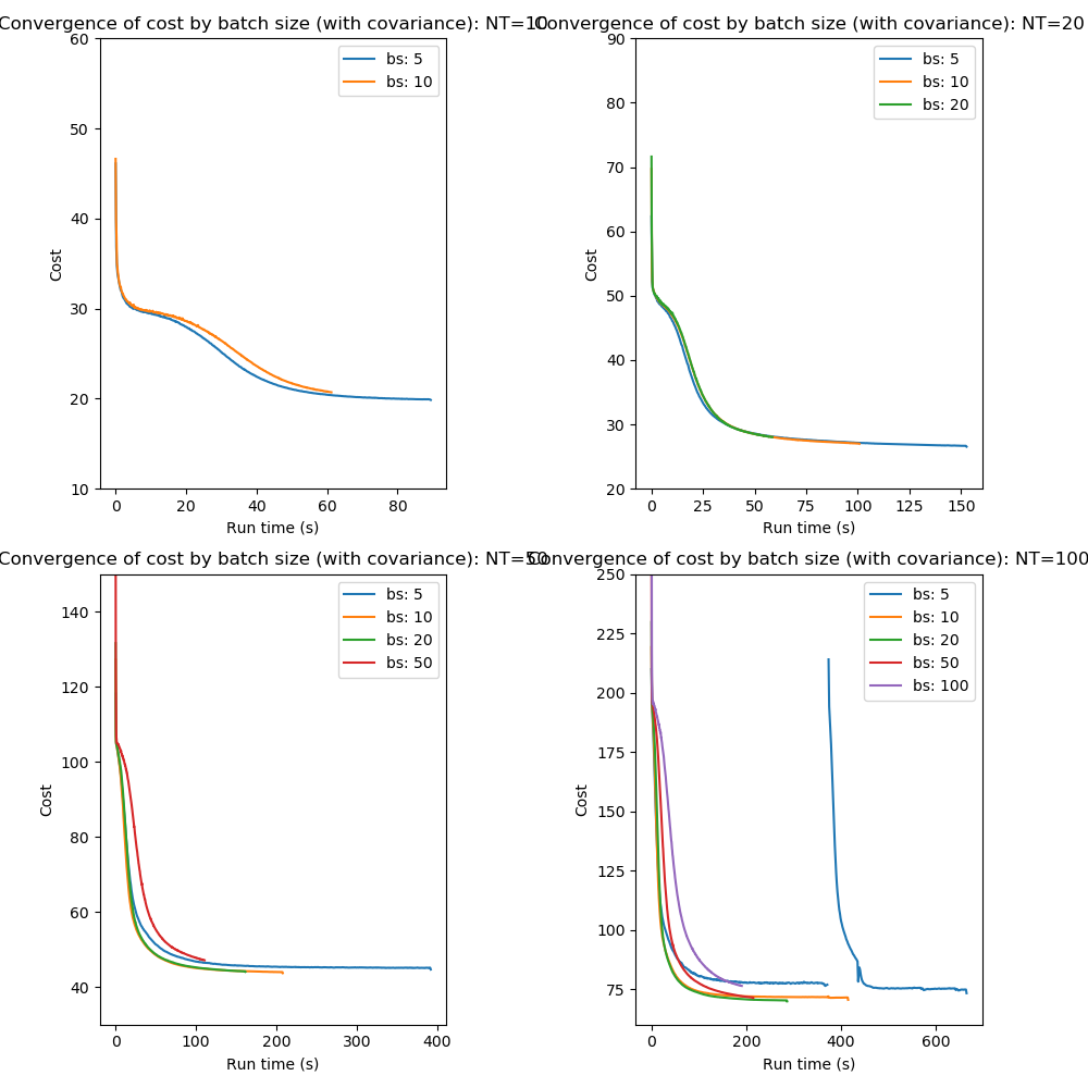
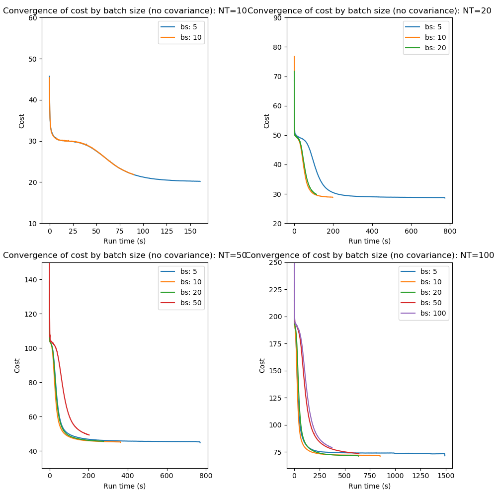
These plots show that mini-batch processing does indeed accelerate convergence especially where the number of data points is high. Batch sizes of 10 and 20 produce consistently fast convergence compared to using the entire data set at each epoch.

Since mini-batch processing increases gradient noise we might expect it to interact with the learning rate which we can investigate by looking at the best cost achieved by learning rate at different batch sizes:

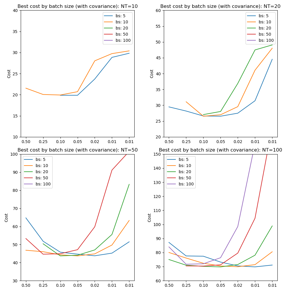
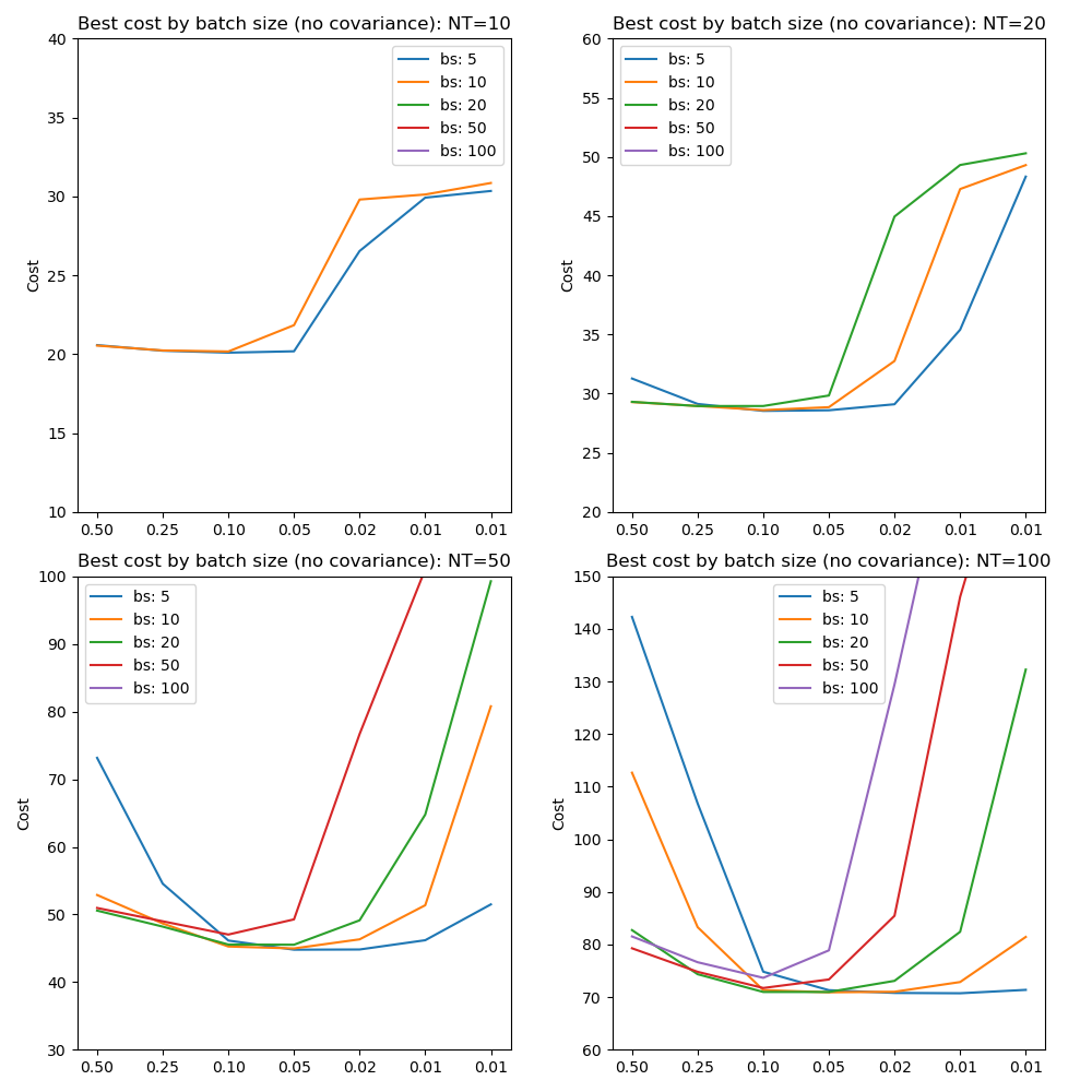
These results confirm the use of learning rates between 0.1 and 0.05 as optimal across batch sizes. In general small batch sizes can be used with lower learning rates. Large batch sizes can reach a lower cost at higher learning rates, although sometimes they are not able to converge at all. This is in line with expectations since high learning rates and low batch sizes both imply a ‘noisier’ optimization and both excessively high or low noise in the optimization can be problematic.

It is noticeable that batch sizes smaller than the number of points in the data only give faster convergence for larger numbers of time points (50 or 100). However there is still an advantage to mini-batch processing in that the best cost curves are ‘flatter’, i.e. more tolerant of variation in the learning rate.

Where batch size is fixed in subsequent tests we use a value of 10.

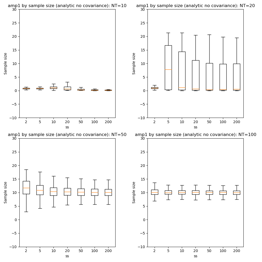
Effect of posterior sample size

The sample size is used to esimate the integrals in the calculation of the cost function, so we would expect that a certain minimum size would be required for a good result. The smaller the sample, the more the resulting cost gradients are affected by the random sample selection which may lead to a noisier optimisation process that may not converge at all. On the other hand, larger sample sizes will take longer to calculate the mean cost giving potentially slower real-time convergence.

Here we vary the sample size with a fixed learning rate of 0.1 and initially without mini-batch processing:

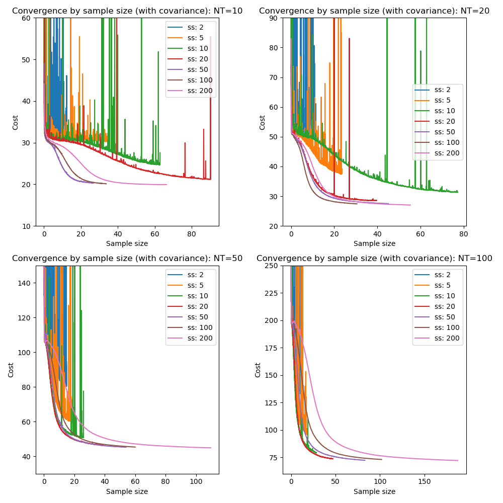
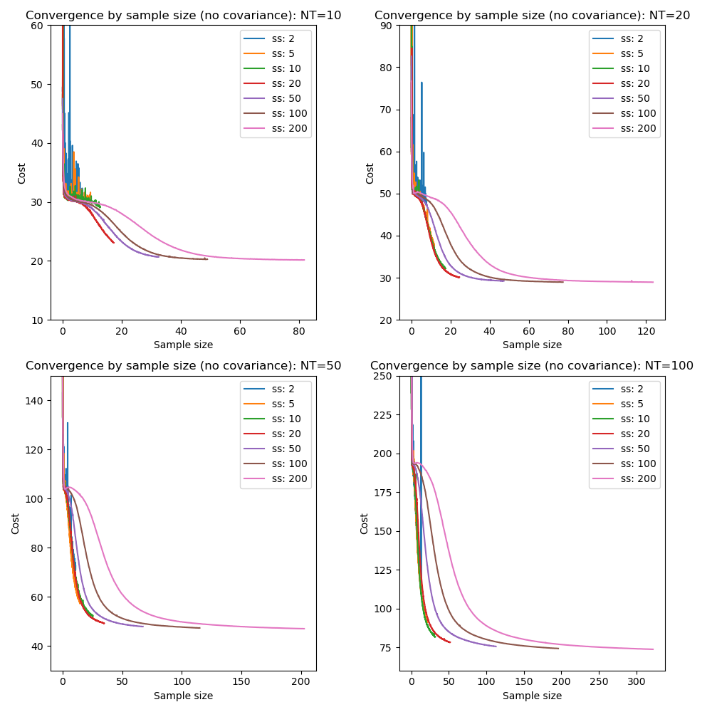
This illustrates that very small sample sizes do indeed result in a noisy potentially non-convergent optimization, and also that larger sample sizes can produce overall slower convergence. The picture is mixed, however the optimal sample size is around 50 when inferring covariance but only 20 without covariance.

We can also look at the equivalent convergence when using mini-batch processing with a batch size of 10:

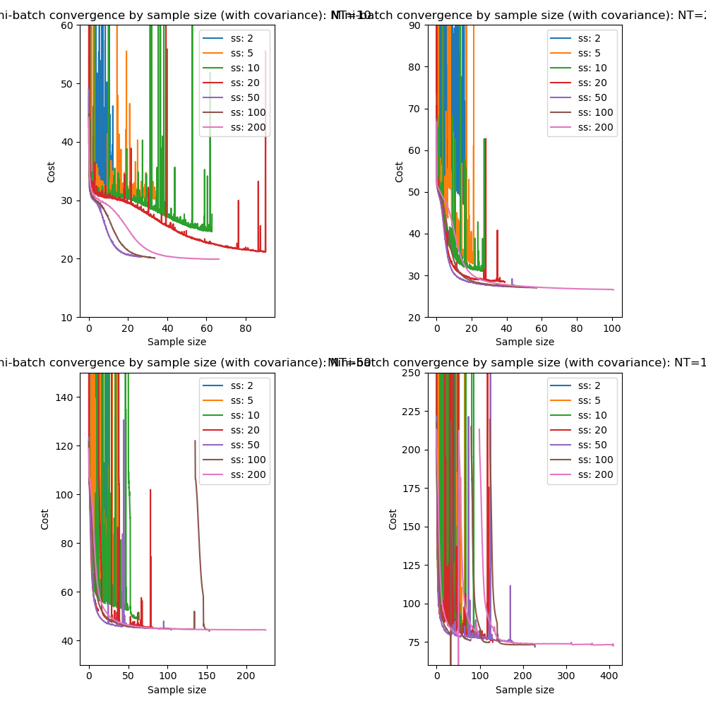
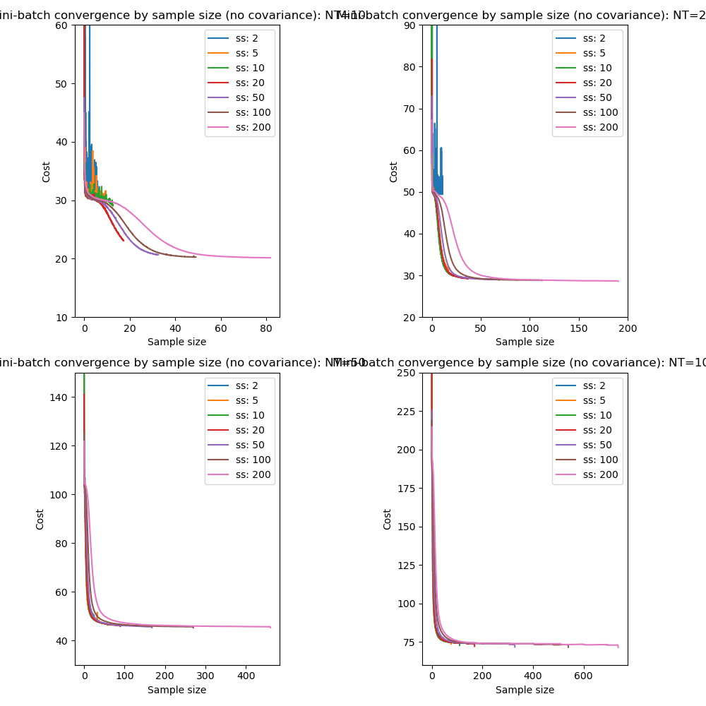
The results are essentially the same however the optimization becomes extremely unstable at small sample sizes when combined with mini-batch processing.

Note also that it is possible that a lower sample size may constrain the free energy systematically (analogously to the way in which numerical integration techniques may systematically under or over estimate depending on whether the function is convex). So the higher free energy of smaller sample sizes does not necessarily mean that the posterior is actually further from the best variational solution.

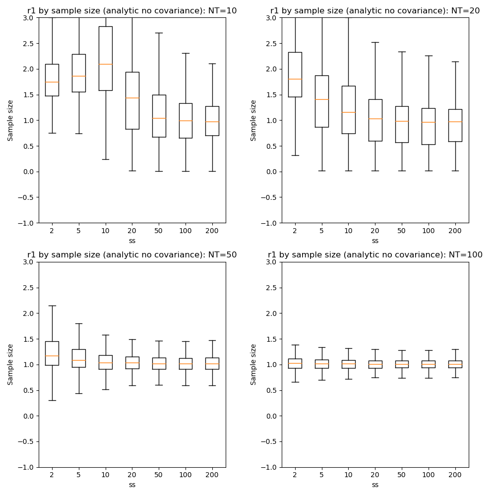
With this in mind it is useful to look at convergence in parameter values (using mini-batch processing as above):

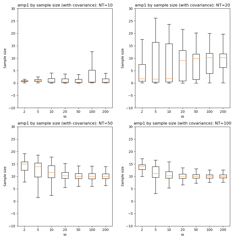
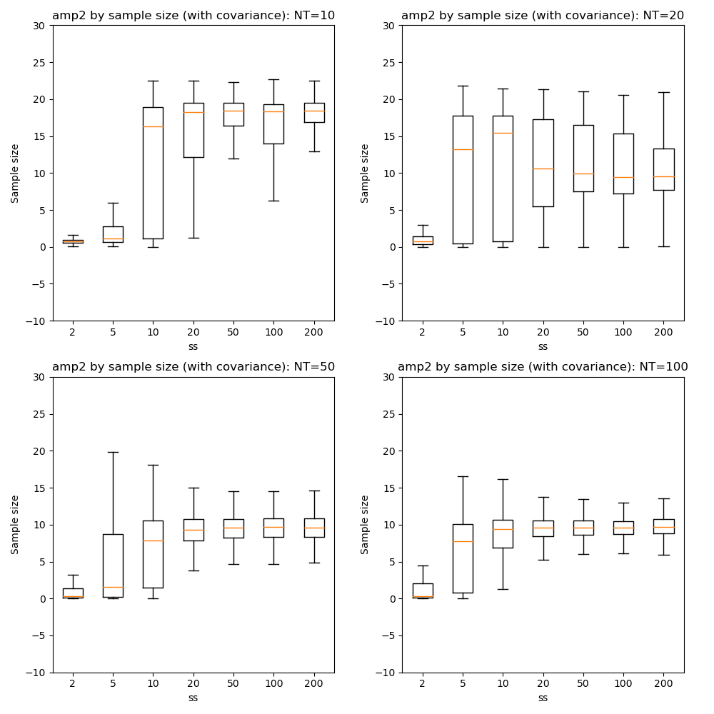
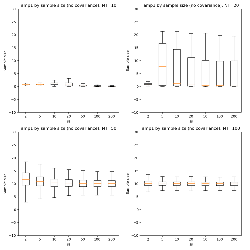
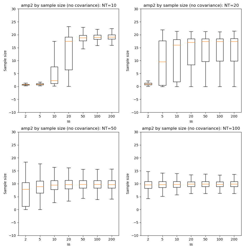
Here we can see that firstly, with fewer data points the optimization tends to favour a single-exponential solution and does not recover the biexponential property for most voxels until we have at NT=50.

In general there is little benefit to sample sizes above 50, and 20 gives very similar results for NT=50 and NT=100.

Effect of prior and initial posterior

The following combinations of prior and posterior were used. An informative prior was set with a mean equal to the true parameter value and a standard deviation of 2.0. Non-informative priors were set with a mean of 1 and a standard deviation of 1e6 for all parameters.

Non-informative initial posteriors were set equal to the non-informative prior. Informative posteriors were set with a standard deviation of 2.0 and a mean which either matched or did not match the true parameter value as described below. In addition, an option in the model enabled the initial posterior mean for the amplitude parameters to be initialised from the data.

Code	Description
i_i	Informative prior, informative posterior initialised with mean values equal to 1.0 for all parameters
i_i_init	Informative prior, informative posterior initialised with true values of the decay rates and with amplitude initialised from the data
i_i_true	Informative prior, informative posterior initialised with true values
i_i_wrong	Informative prior, informative posterior initialised with mean values of 1.0 for the decay rate and 100.0 for the amplitudes (i.e. very far from the true values)
i_ni	Informative prior, non-informative posterior
i_ni_init	Informative prior, non-informative posterior with amplitude initialised from the data
ni_i	Non-informative prior, informative posterior initialised with mean values equal to 1.0 for all parameters
ni_i_init	Non-informative prior, informative posterior initialised with true values of the decay rates and with amplitude initialised from the data
ni_i_true	Non-informative prior, informative posterior initialised with true values
ni_i_wrong	Non-informative prior, informative posterior initialised with mean values of 1.0 for the decay rate and 100.0 for the amplitudes (i.e. very far from the true values)
ni_ni	Non-informative prior, non-informative posterior
ni_ni_init	Non-informative prior, non-informative posterior with amplitude initialised from the data

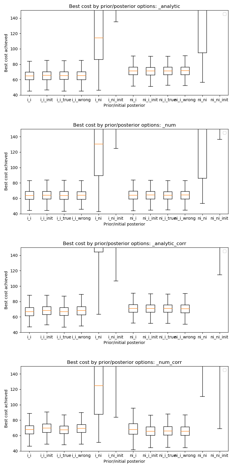
These results show that in terms of absolute convergence there is no significant difference between the choice of prior and posterior. Note that the absolute cost achieved can be different between the informative and non-informative priors as expected. The exception is the cases where a non-informative initial posterior is used - these cases do not achieve convergence.

The explanation for this lies in the fact that components of the cost are dependent on a sample drawn from the posterior. In the case of a non-informative posterior samples of realistic sizes cannot be large enough to be representative and different samples may contain widely varying contents. Such samples cannot reliably direct the optimisation to minimise the cost function because the calculated cost (and its gradients) are dominated by random variation in the values contained within the sample.

By contrast if the posterior is informative - even if it is far from the best solution - different moderately-size random samples are all likely to provide a reasonable representation of that distribution. The optimisation will therefore be directed to minimse the cost more reliably since it is less dependent on the particular values that happened to be included in the sample.

We conclude that the initial posterior must be informative even if it is a long way from the true solution.

The _analytic and _num plots are identical apart from using the analytic or the numerical solution to the KL divergence between two MVNs. The similarity between these results suggests that the numerical solution should be sufficient in cases where the prior and posterior cannot be represented as two MVN distributions.

The _corr and __nocorr plots were generated with and without a full posterior covariance matrix. In this case we see little difference between the two.

It is reassuring that the cost can converge under a wide variety of prior and posterior assumptions, however it is also useful to consider the effect of these variables on speed of convergence. The results below illustrate this:

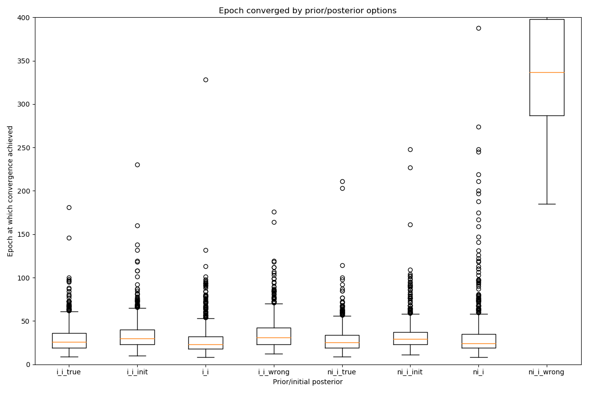
This plot shows the epoch at which each voxel converged (to with 5% of its final values). The box plot show the median and IQR, while the circles show slow-converging outliers. For the reasons given above, non-informative posterior test cases were excluded from this plot.

It is clear that the main impact on convergence speed is the initial posterior. Where it is far from the true values (i_wrong) convergence is slowest. However this problem is much less obvious when the priors are informative as in this case the ‘wrong’ posterior values generate high latent cost as they are far from the ‘true’ prior values. This quickly guides the optimisation to the correct solution. Initialisation of the posterior from the data (where there is a reasonable method for doing this) is therefore recommended to improve convergence speed.

Numerical vs analytic evaluation of the KL divergence

In the results above we have used the analytic result for the KL divergence of two multivariate Gaussian distributions. In general where the posterior is not constrained to this distribution we need to use a numerical evaluation which involves the posterior sample. So it is useful to assess the effect of forcing the numerical method in this case, particularly in combination with variation in the sample size.

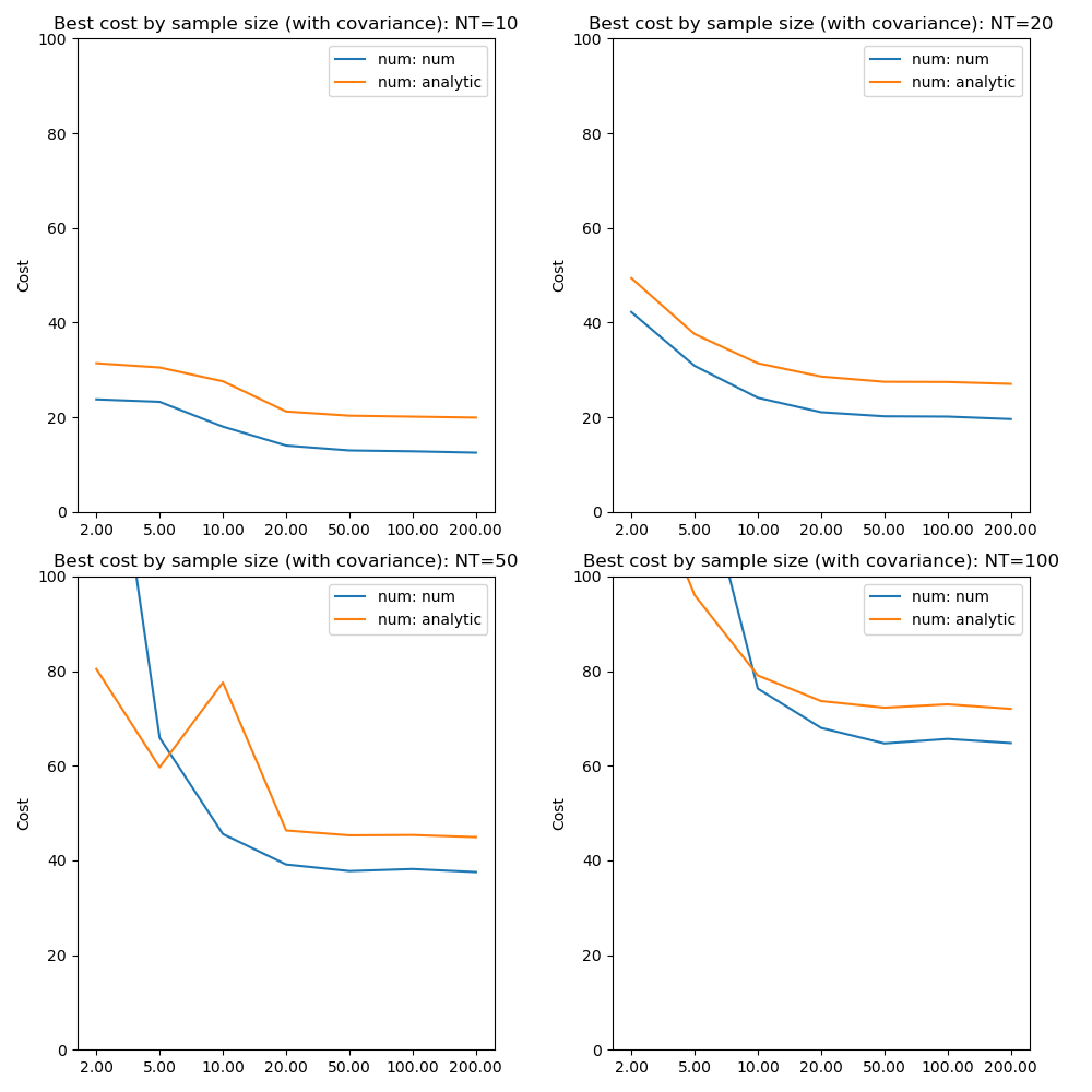
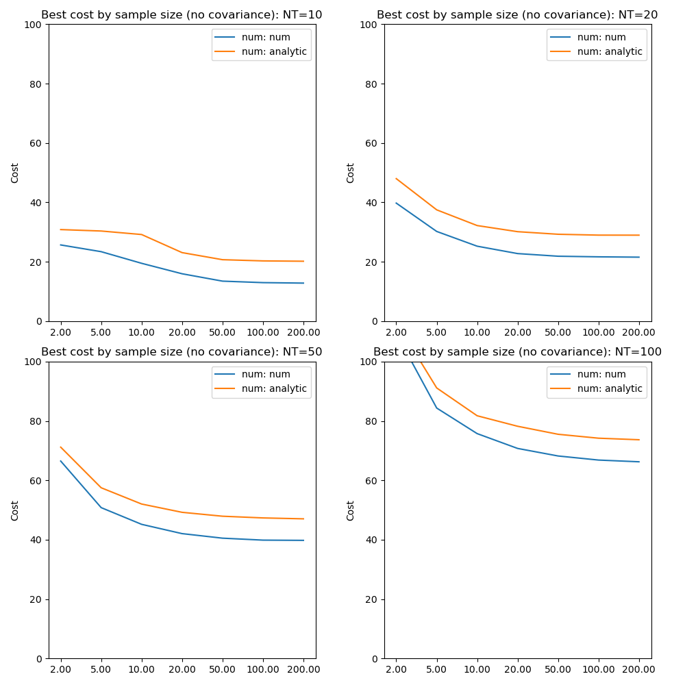
The absolute values of the free energy cannot be compared directly since some constant terms in the analytic solution are dropped from the calculation. The convergence properties with sample size, however, are closely similar even though part of the cost is independent of sample size in the analytic case.

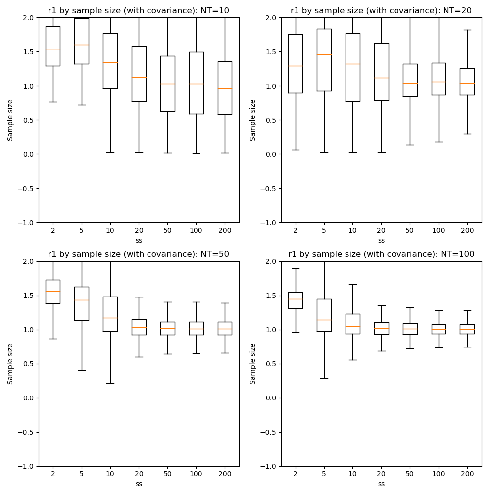
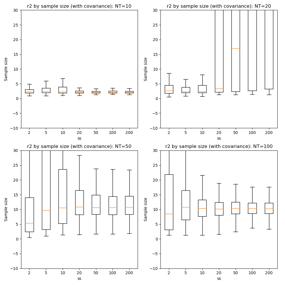
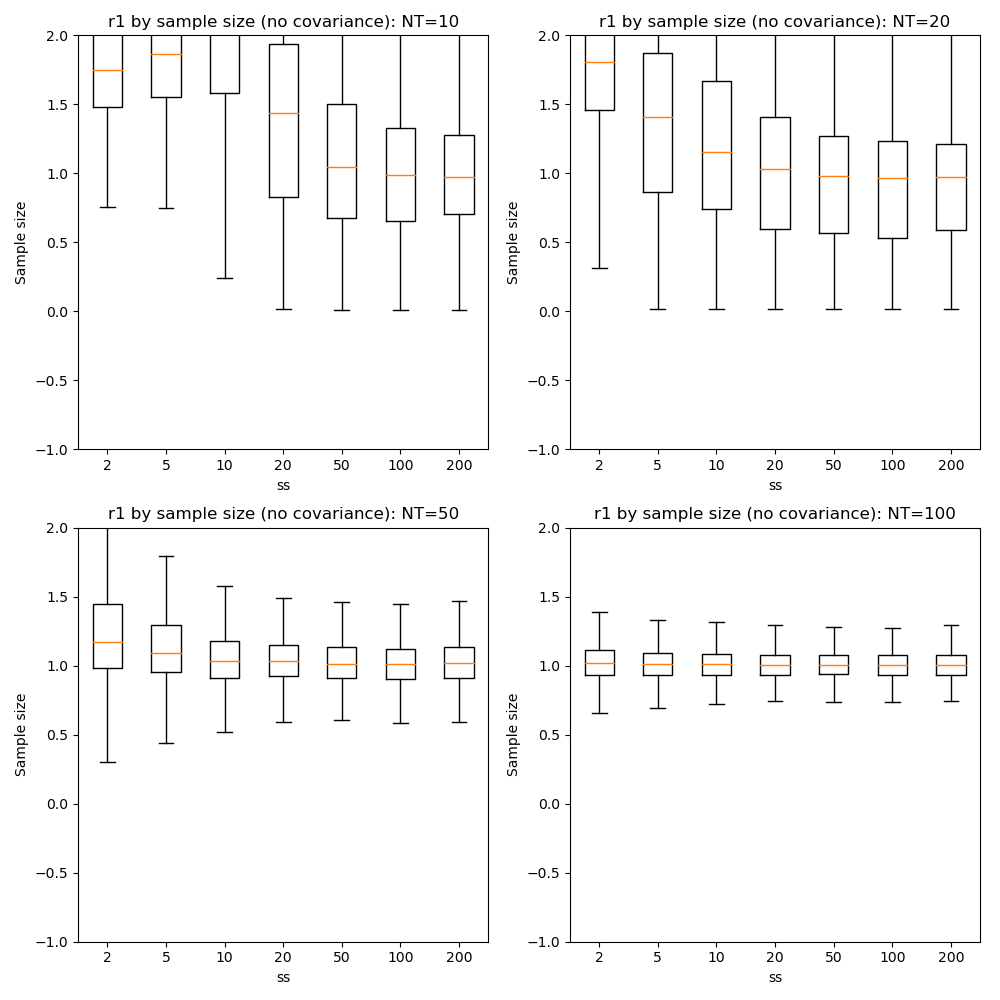
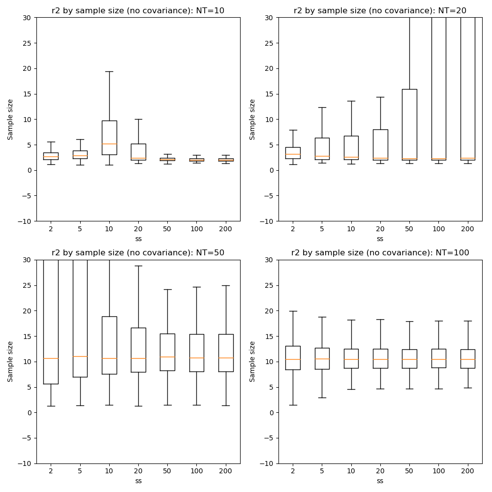
We can also compare parameter convergence with sample size:

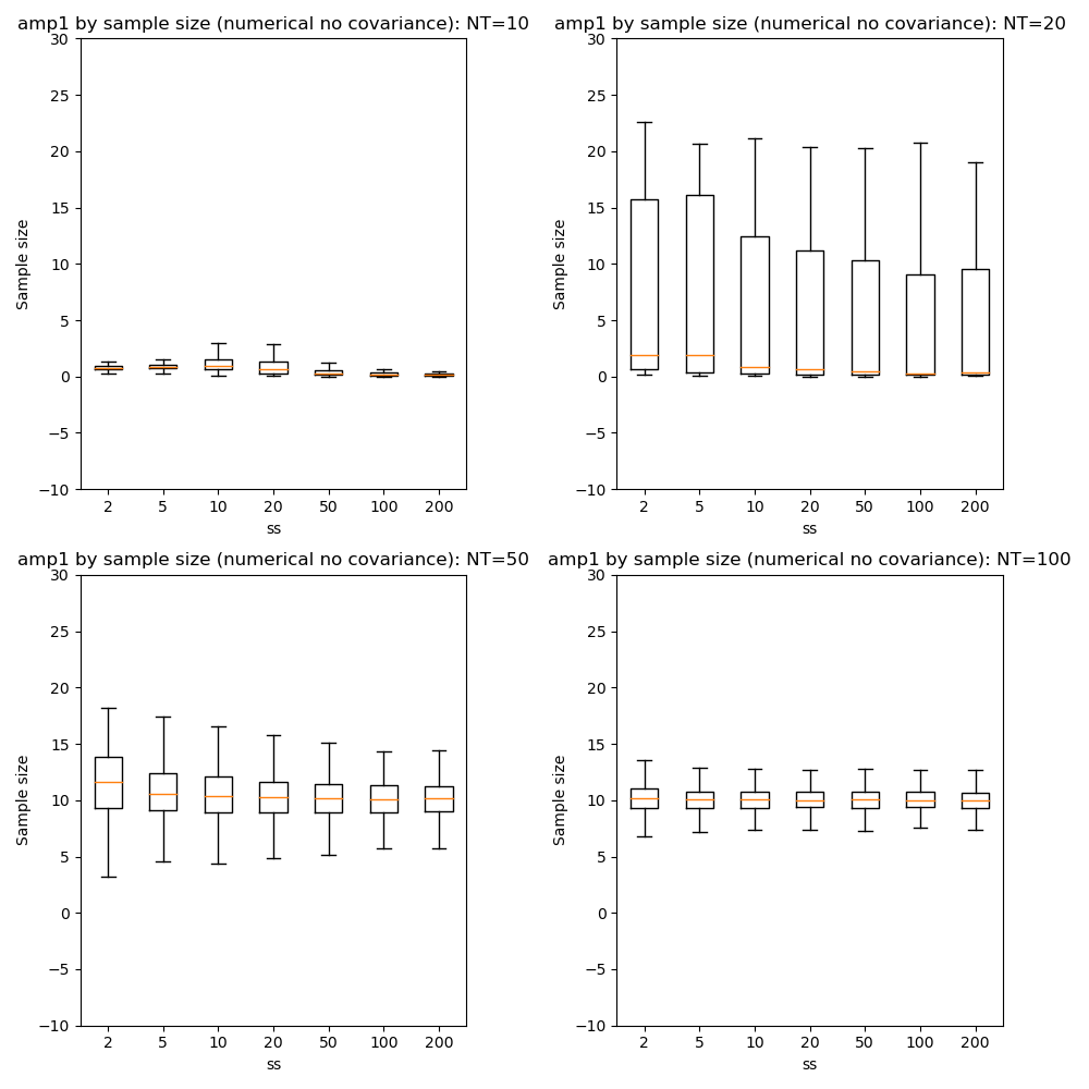
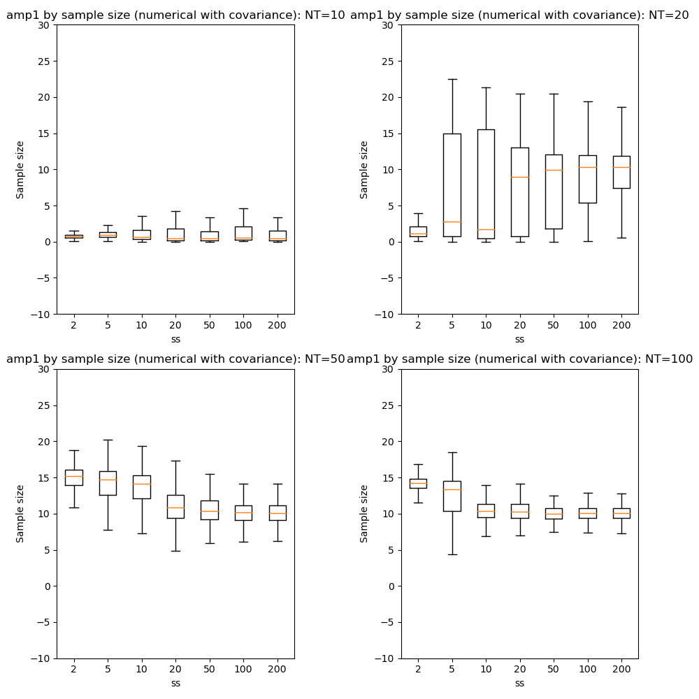
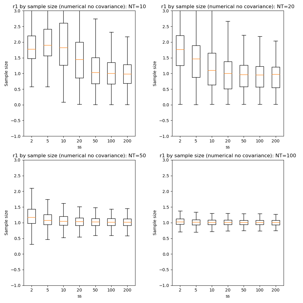
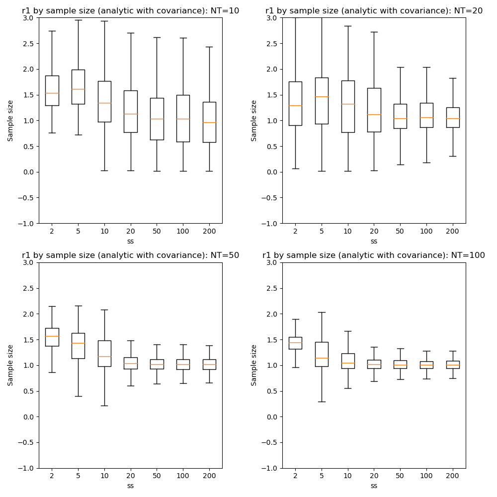
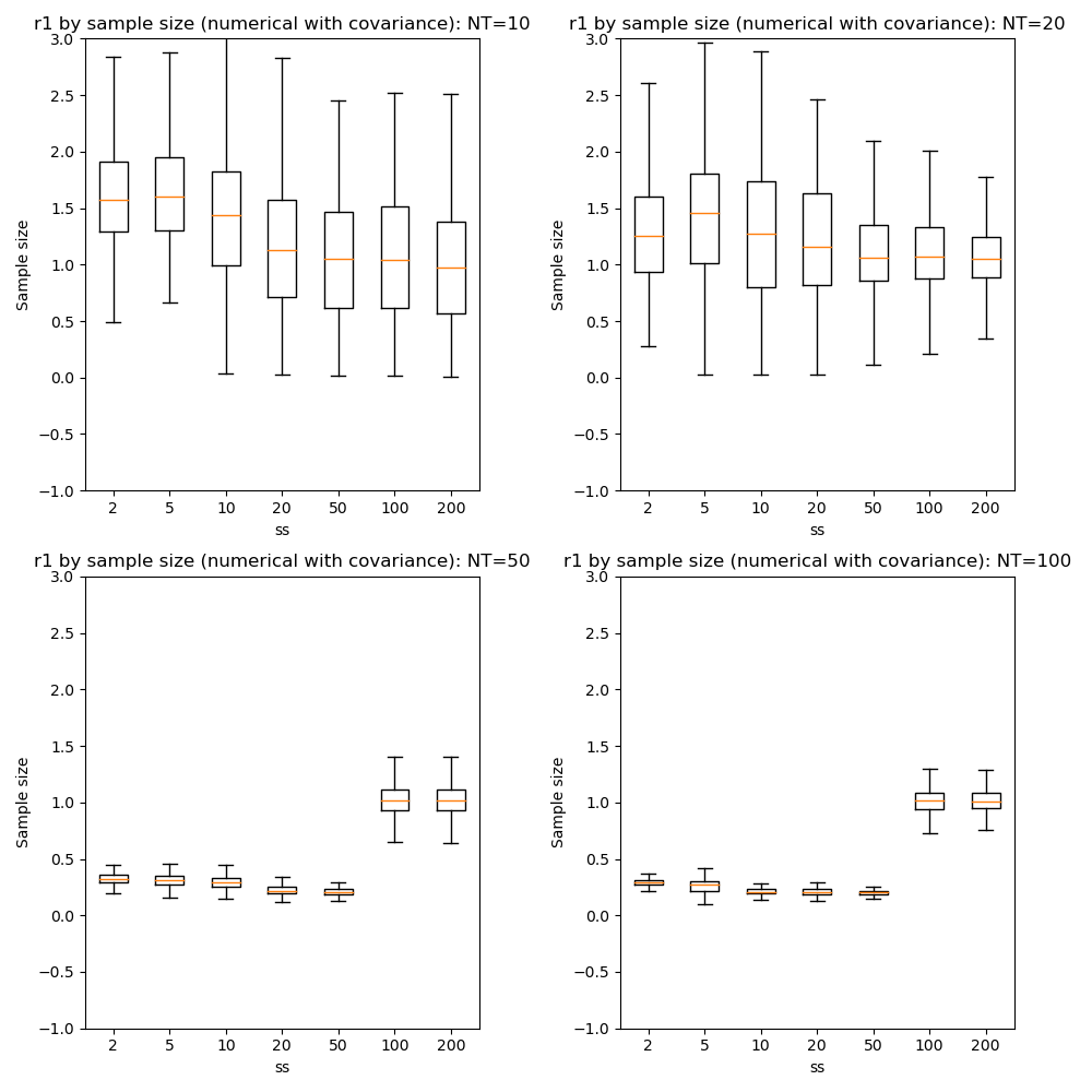
In most cases the numerical and analytic solutions seem very similar, however in the case of the rate parameter we do not appear to get a converged result at NT=50 or 100 until we have a sample size of 100 when inferring covariance. This requires additional investigation since it is out of step with the remainder of the results.

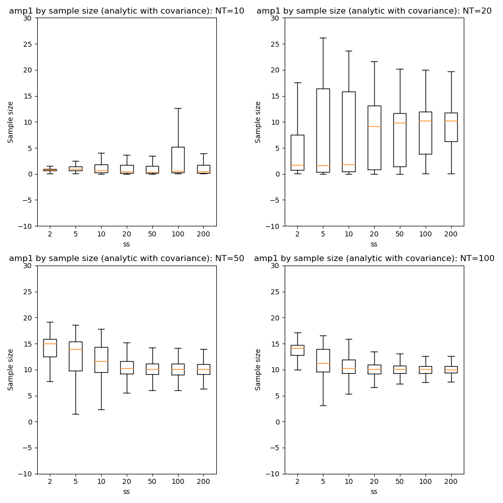
Inference of covariance

The effect of inferring covariance or not has been shown throughout these tests. In general the effect is that convergence is more challenging with covariance as would be expected with the increased parameter space, and instabilities caused by small batch or sample sizes, or large learning rates, are exacerbated by the inclusion of covariance. It’s worth mentioning that the symmetry of the biexponential model would expect to generate significant parameter covariances.

A strategy of initially optimizing without covariance, and then restarting the optimization with the covariance parameters included is an obvious way to address this.